The Effects of Transfer Learning on Medical Imaging

To View the Source Code Click Here!
Diabetic Retinopathy (DR) is one of the leading causes of blindness for working-age adults. As a competition, Aravind Eye Hospital in India has asked the community of Kaggle to help them find an algorithm that will help them screen for DR. Currently, technicians must travel to these rural areas to take the images which then must be reviewed by highly trained doctors to diagnose DR.
The task in the competition is to develop a predictive algorithm that would be able to help doctors scale their efforts to detect and treat DR. The APTOS problem can be broken down into two main parts: part one, does the subject have DR; and part two, if the subject has DR what how severe is it? The primary goal for this problem is not necessarily to beat human recognition of the condition, but to create an algorithm that can assist in scaling the efforts of hospitals in treating DR through increased detection rates. Solutions found to this problem will then be spread to other Ophthalmologists throughout the Asia Pacific Tele-Ophthalmology Society (APTOS) Symposium.
Transfer learning has become an industry-standard in computer vision problems, and a favored technique among Kagglers. Transfer learning saves time and resources which all equate to money saved. Transfer learning happens when a pre-built model is re-trained for another purpose. For example, this research is taking models that have been pre-trained on ImageNet, a database with over 14 million labeled images, and retraining these models to detect DR. Transfer Learning is effective because all images share similar qualities and therefore, what these models have previously learned can be re-used. Previous winners of the APTOS competition have used DenseNet, EfficientNet, and ResNet for transfer learning, but how do these models compare? The objective of this paper is to understand how effective transfer learning is in medical imaging, and furthermore, how the various established transfer learning models compare when they are exposed to medical images.
To understand and answer this question, our research will be broken down into four sections: Description of the Data, Comparing Transfer Learning Techniques, Tuning the Best Model, and Results. Description of the Data will discuss how the data is organized and the image preprocessing pipeline. Comparing Transfer Learning Techniques will discuss the methodology used to compare transfer learning models and how we evaluated their performance. After comparing the various transfer learning techniques, the next section, Tuning the Best Model, will further tune the best performing transfer learning model.
Description of the Data
The dataset provided contains 4,000 colored images of retinas and is approximately 10GB in size. Each image is labeled one of five class, and they are as follows: No DR, Mild DR, Moderate DR, Severe DR, and Proliferative DR. These images are all stored in PNG format and vary in size, resolution and quality. This section will be broken down into three parts: Class Balance, Image Quality, and Image Preprocessing. Part one will describe the different classes and how these classes are balanced. Part 2 will discuss image quality and some of the key signs of DR. Part three will discuss the image preprocessing pipeline.
Class Balance:
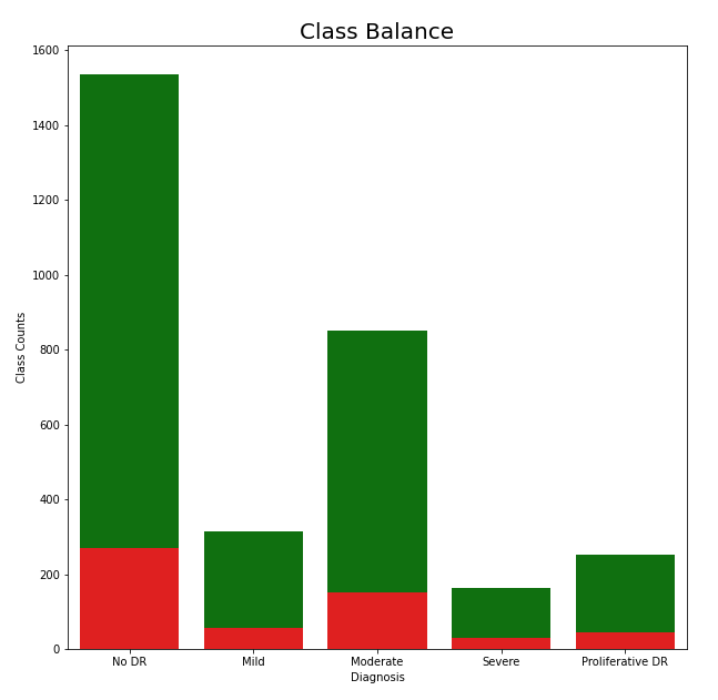 As previously mentioned, each image belongs to one of five classes, and the balance of these classes can be found in the chart to the left. When looking at the classes from a binary classification point of view, those who do have DR and those who don’t, the data seems to be well balanced. However, when looking at the distribution of cases for the degrees of DR, the classes become unbalanced. To account for this, we used class weights to adjust for class imbalance. This allowed our cost function, categorical cross-entropy, to account for the unequal distribution of classes. Furthermore, the test split is also shown in the diagram which is colored red. The test split is shown to be representative and it should capture the overall structure of the data.
Image Quality:
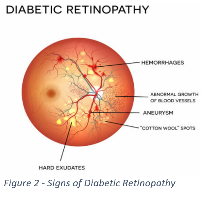
When determining if a subject has DR and how severe a case is, a doctor will look for several key signs such as hemorrhages, aneurysms, and “Cotton Wool” spots, which can be seen in Figure 2. Below in Figure 3, we can see images associated with each individual class, and each one of the images shows at least one of the several key signs. These signs can be difficult to detect, for some images are too dark to make out details, or smaller parts of an image can get lost in the background. This led us to look for a way to preprocess our data to increase its readability.

Image Preprocessing:
 In order to make our training as effective as possible we explored several ways to change our dataset to improve the readability of our images. We transformed our images into black and white, black and white images with Gaussian Blur, and color images with Gaussian Blur. Gaussian Blur is a technique that softens images in a way that removes extraneous edges and allows for more accurate edge detection in an image. The previous winners of the competition used Gaussian Blur on black and white images, but since then it has been shown that using Gaussian Blur on color images can produce even better results. As such, we chose to use color Gaussian Blur to preprocesses our images. The clear differences in visibility and readability after using colored Gaussian Blur can be seen in Figure 4. When comparing figures 3 and 4, troubled areas such as ‘Cotton Wool Spots’ have become more pronounced and easier to identify. As previously mentioned, exposer or lighting is also an issue, and Gaussian Blur seem to have taken care of this.
To ensure that our models would generalize to unseen images, this research made use of image generators. Image generators add noise as they go through training which allows the model to generalize better on unseen images. Some of the image transformation used were picture rotation, height and width shift, sheer, and zoom. Image generators ensured that our models do not become too fixated on certain patterns or locations within an image. The image transformations found in figure 5 allowed our model to tell what should and shouldn’t be in a retina image no matter the orientation, size, or color.
Comparing Transfer Learning Techniques

To tackle the problem facing us, we decided to use a convolutional neural network (CNN) built with transfer learning models. We utilized several different kinds of models and compared them to determine which was best. These models, unlike ones from previous competitions, are comparable as they were all trained using ImageNet. The flow diagram above shows the overall process for finding the best transfer learning model. Once we determined the most effective model, we then began fine-tuning it to get our final results.
Each of these different transfer learning models in the flow diagram above offers up a different way to approach the problem at hand. VGG19 runs a model that sets many parameters of a model and pushes the depth to 19 layers. This is possible due to using small (3X3) convolution filters in all layers of the model, and allows for increased accuracy . ResNet allows for very deep models while avoiding the usual pitfalls of vanishing gradients and the degradation of training accuracy. It does this by using normalized initialization (for vanishing gradients) and by implementing a deep residual learning framework that explicitly allows new layers of a model to fit residual mapping. This is accomplished by adding connections, known as skip connections, that perform identity mapping, these outputs are then added to the outputs of stacked layers in the model. DenseNet models adds even more identity connections between layers than ResNet and uses the outputs of previous layers as inputs. This set up allows DenseNet to require fewer parameters and have a type of “collective knowledge” throughout the model to which individual layers contribute. CNNs are often scaled up only when there are enough resources available, EfficientNet looks to increase the efficiency of scaling a neural network so this can happen more readily. EfficientNet scales the depth, width, and resolution of a CNN uniformly using a compound coefficient based on constants determined using a small grid search on the original smaller model. Xception is a model that takes its inputs and breaks them down so that it maps correlations for each input channel separately, then uses a 1X1 convolution to capture correlation across channels. Xception is built off a previous model called InceptionV3, and uses the same number of parameters, showing that the new structure more efficiently uses whatever parameters are input into the model.
 Due to the existing training and finetuning of the transfer learning models on ImageNet we only wanted to train some of the end layers in our models. The earlier layers in transfer learning models are capturing more generic and abstract concepts of images such as shapes. The later layers are where the specifics and context of an image can come out in training. Due to this, we chose to unfreeze the last 5 layers of these pre-trained models to allow for the specific context of our retina images to be trained into the model. Unfreezing only the first five layers does present issues when trying to compare these transfer learning models because they have different structures but due to time restrictions and resources it was decided to only unfreeze the last five layers. Only unfreezing five layers significantly decreased the amount of trainable parameters which in the end saves time.
Our first initial layer after the transfer learning model was either a flattening layer or a Global Pooling layer. If a model we were running had more than 10 million total trainable parameters (several had parameters approaching 25 to 30 million) we used Global Average Pooling to reduce the total number of trainable parameters. For each of the transfer learning models we set up a CNN back end that utilized three blocks which contained batch normalization, dropout and a Relu dense layer (see figure 9). A SoftMax layer was used as an output layer do to this problem being a multiclass classification problem, but it should be said that several kagglers, with success, have used mean squared due to the classes being ordinal.
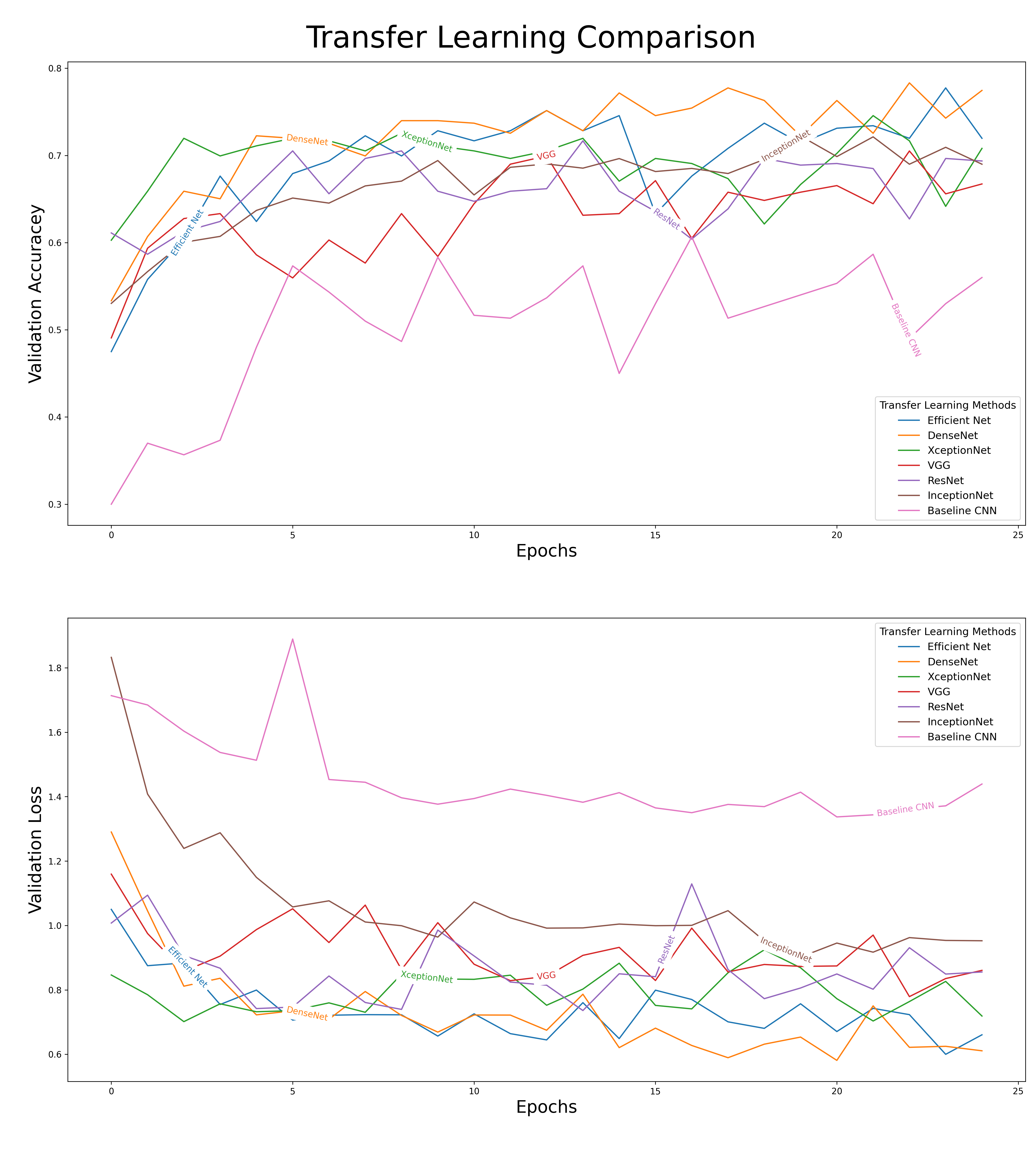
Essential, every transfer learning model had its last five layers unfrozen and were fitted with similar backends, and this allowed us to compare their results. When we compare the results of our different models, there was a clear difference in their performances. As shown in figure 8, the effects of transfer learning can clearly be seen in our baseline CNN (a model not equipped with any transfer learning model). The baseline CNN drastically underperformed when compared to the other models. We decided to move forward with DenseNet as our primary model for fine-tuning. A comparison of the outputs from our different models can be seen below.
Tuning the Best Model
 To fine-tune our DenseNet model, we cycled through several different parameters. The first hyperparameter we decided to tune was the learning rate. The output from the various models in the transfer learning section seemed to need a lower learning rate then the default values. To tune the learning rate, we ran models which had a learning rate of .01, .001 and .0001. After running through the various learning rates, it was determined that a learning rate of .0001 seemed to work best. After determining the best learning rate, this research employed a 3-block design to determine depth, width, and activation function.
 Figure 9 shows the basic structure of our nueral network blocks. Each block contains batch normalization, drop out and one dense layer. Our largest model contained three blocks while our smallest model contained only one block. As the number blocks increased within a model the number of neurons decreased within size (layer 1 - 500, layer 2 - 100, and layer 3 - 32). For tuning the activation function, we chose to stay within the ReLu family, and so we also changed the dense layers to either ReLu, SeLu, or Elu. The table to the right shows the top-performing model from this hyperparameter tuning exercise.
Results and Conclusion
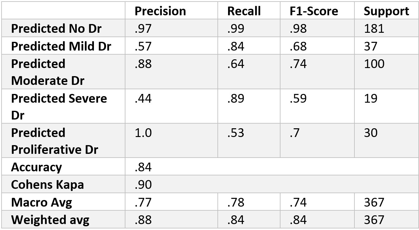

We found that the 1-block Elu (1Elu) combination of parameters was our most effective option. The results from this combination can be found in the table above. As shown in the confusion matrix, the model did very well in distinguishing between patients with DR and patients without DR. As expected, the different ranges of severity of DR did not do as well. The most troubling category is Severe DR, for half of its class fell into the moderate category. Although there is room for improvement, the model performed well. For the most part, when the model makes a mistake it is only by one level (i.e. classifying a severe case as a moderate). Cohen’s Kappa, which is able to account for class order, captures this observation for it shows almost perfect agreement between the two raters, which in our case are actual and predicted values. Since the model seems to be doing well with class order, perhaps future studies could convert this into a regression problem and not a classification problem.
We could have used Quadratic Cohen’s Kappa as a better metric when evaluating our models during training; although we did measure it in our final model. Cohen’s Kappa compares two raters’ results (in our case our model and the actual result) and calculates the reliability of the two ratings, corrected for how often the raters might agree by chance. This metric would have also considered the inherent order of the classes and would have given a smaller penalty to results that only differed from one level. Due to issues with the Keras library, we were unable to monitor Cohen’s Kappa throughout training, but did consider it in the final model.
We did run into some limitations in our implementation of our model. We chose 25 epochs as our limit to run our different models on and after analyzing our results we believe that there is room for improvement in running more epochs for our models. We could have also experimented with increasing the image size, we resized everything to 224x224. Increasing the size of the image could have provided more information to model and therefore increase performance. An improvement we could have made to our preprocessing of the data is to have cropped out useless parts of our images. When we resized our images, we just simply forced all the images to 224x224, but applying a more stringent cropping method could have cropped out useless areas and therefore saved image quality during re-sizing.
In the transfer learning comparison section, how we chose to unfreeze transfer learning layers could have also been improved. The structure of these transfer learning models differs, and because we chose to only unfreeze the last five layers of each transfer learning model, comparing the models presents issues. An alternative to this would be to have unfrozen all layers from the beginning, but we did not go this route due to time restrictions and resources available. When fine-tuning the best model (ie DenseNet), we could have gone through a systematic check when unfreezing our layers during the fine-tuning process, (ie checking 5 layers, then 10, and so on).
In summary, the results of this exercise clearly show the power of transfer learning in the medical imaging landscape. Medical Images are radically different from a normal image, but even with this, our final model did exceptionally well. This truly shows the unbounded flexibility of transfer learning. This exercise also revealed the importance of image preprocessing. Preprocessing the images by using Gaussian Blur not only made training the model faster but also more accurate. In conclusion, transfer learning is a powerful, flexible method in the medical imaging landscape.